Single exposure models

Single exposure models focus on the evolution of surface coverage with time under different experimental conditions. Here is a list of currently implemented and in development models. They are all based on models published in the literature.

0D constant partial pressure model

The ZeroD model implements the simplest possible case in ALD: the evolution of surface coverage as a function of exposure for a constant partial pressure pulse:

from aldsim import Precursor, ALDchem
from aldsim.models import ZeroD
import matplotlib.pyplot as pt

# Define a precursor (TMA with molecular mass in g/mol)
tma = Precursor('TMA', mass=144.17)

# Define surface kinetics with ideal Langmuir behavior
kinetics = ALDchem(prec=tma, nsites=1e19, p_stick1=0.01)

# Create the ZeroD model at 200°C and 100 Pa
model = ZeroD(chem=kinetics, T=473.15, p=100)

# Generate the saturation curve
time, coverage = model.saturation_curve()

# Plot the saturation curve
pt.plot(time, coverage)
pt.xlabel("Dose time, s")
pt.ylabel("Fractional surface coverage")
pt.show()

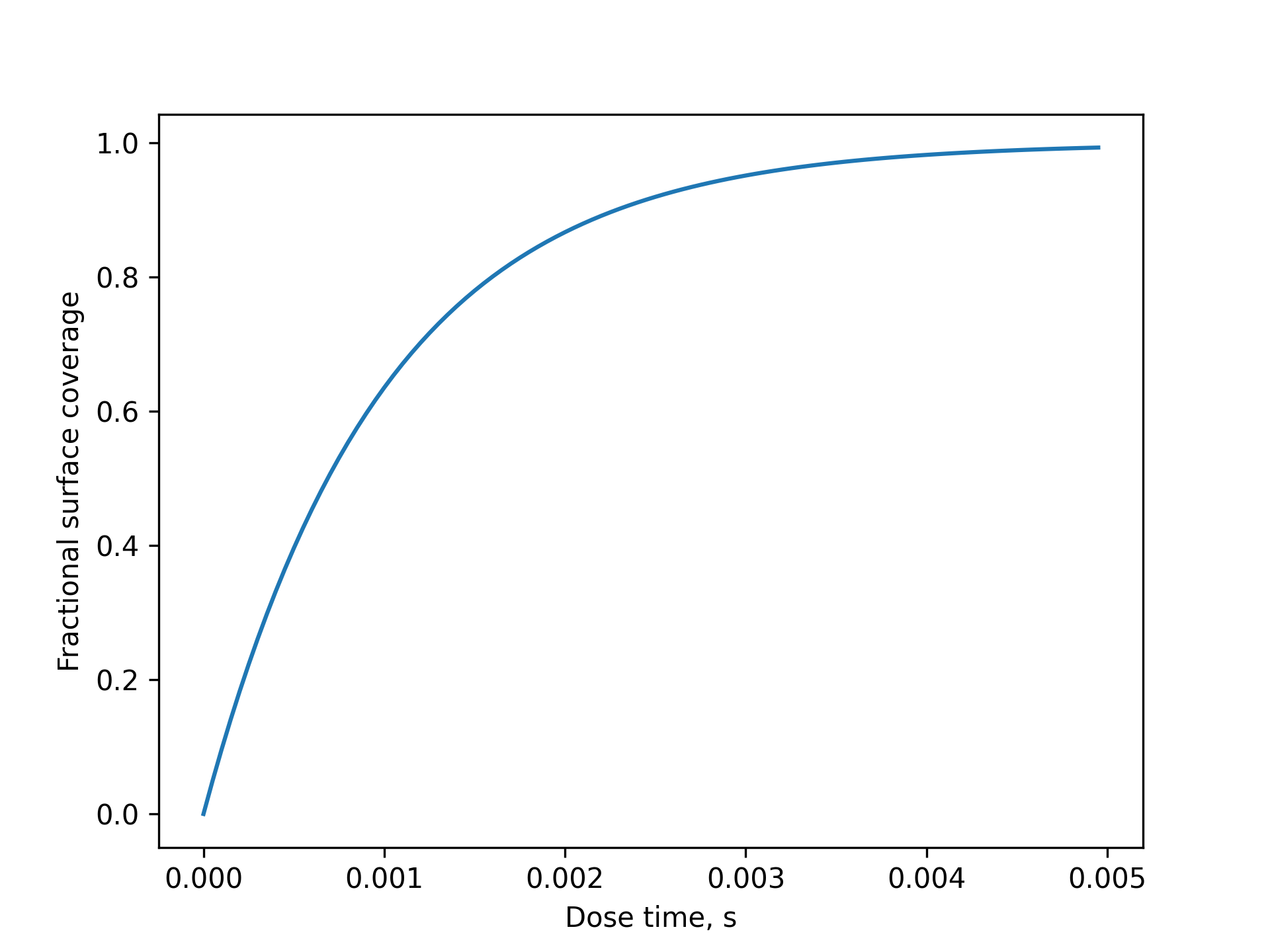
Saturation curve for the ZeroD model.

ALD of particles in fluidized bed reactors

Note

The FluidizedBed model is currently implemented for ALD surface kinetics with a single reaction pathway only. Use ALDchem for the surface chemistry definition.

The model for ALD in a fluidized bed reactor is directly implemented from the works:

• Scalable synthesis of supported catalysts using fluidized bed atomic layer deposition

• Modeling scale-up of particle coating by atomic layer deposition. A preprint is available in arXiv

This model considers a perfectly mixed column of particles and a plug flow model for precursor transport across the column:

from aldsim import Precursor, ALDchem
from aldsim.models import FluidizedBed
import matplotlib.pyplot as pt


# Define precursor and surface chemistry
tma = Precursor('TMA', mass=144.17)
chem = ALDchem(tma, nsites=1e19, p_stick1=1e-3)

# Create the FluidizedBed model
# p: precursor partial pressure (Pa), p0: carrier gas pressure (Pa)
# T: temperature (K), S: total particle surface area (m²), flow: gas flow (sccm)
model = FluidizedBed(chem, p=13.2, p0=100, T=500, S=10, flow=60)

# Generate the saturation curve
time, coverage = model.saturation_curve()

# Plot the saturation curve
pt.plot(time, coverage)
pt.xlabel("Dose time, s")
pt.ylabel("Fractional surface coverage")
pt.show()

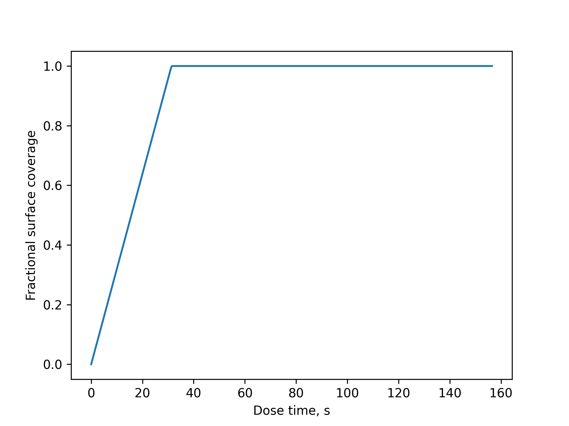
Saturation curve for the FluidizedBed model.

Todo

Add support for soft saturating ALD processes.

Todo

Add support for plasma based processes.

ALD of particles in a rotating drum reactor

Note

The RotatingDrum model is currently implemented for ALD surface kinetics with a single reaction pathway only. Use ALDchem for the surface chemistry definition.

Model for particle coating on a well-stirred environment as described in:

• Analytic expressions for atomic layer deposition: Coverage, throughput, and materials utilization in cross-flow, particle coating, and spatial atomic layer deposition

• Modeling scale-up of particle coating by atomic layer deposition. A preprint is available in arXiv

This model considers a perfectly stirred reactor model for particle coating using ALD:

from aldsim import Precursor, ALDchem
from aldsim.models import RotatingDrum

prec = Precursor(mass=150.0)
nsites = 1e19
p_stick1 = 1e-3
chem = ALDchem(prec, nsites, p_stick1)

# Create the RotatingDrum model
# p: precursor partial pressure (Pa), p0: carrier gas pressure (Pa)
# T: temperature (K), S: total particle surface area (m²), flow: gas flow (sccm)
model = RotatingDrum(chem, p=0.1*1e5/760, p0=1e2, T=500,
               S=1e1, flow=60)

t, theta = model.saturation_curve()

Saturation curve for the RotatingDrum model.

Todo

Add support for soft saturating ALD processes.

Spatial ALD reactor model

Note

The SpatialWellMixed model is currently implemented for ALD surface kinetics with a single reaction pathway only. Use ALDchem for the surface chemistry definition.

Model for ALD coating in a spatial reactor using a well-stirred precursor approximation. This model supports two configurations:

• Flat surface coating: When S is None, the model treats the substrate as a flat surface with area L × W (e.g., roll-to-roll coating of flexible substrates).

• Particle bed coating: When S is provided, it represents the total surface area of particles to be coated within the reactor zone. Particles are assumed to be well mixed in the directions perpendicular to the movement (i.e. by vibrating bed or other agitation methods)

The model is described in the following papers:

• Analytic expressions for atomic layer deposition: Coverage, throughput, and materials utilization in cross-flow, particle coating, and spatial atomic layer deposition

• Modeling scale-up of particle coating by atomic layer deposition. A preprint is available in arXiv

The saturation curve is expressed as a function of web/substrate velocity:

from aldsim import Precursor, ALDchem
from aldsim.models import SpatialWellMixed
import matplotlib.pyplot as pt

# Define precursor and surface chemistry
prec = Precursor(mass=150.0)
chem = ALDchem(prec, nsites=1e19, p_stick1=1e-3)

# Create the SpatialWellMixed model for flat surface coating
# p: precursor partial pressure (Pa), p0: carrier gas pressure (Pa)
# T: temperature (K), flow: gas flow (sccm)
# L: zone length (m), W: zone width (m)
model = SpatialWellMixed(chem, p=13.2, p0=100, T=500,
                         flow=60, L=0.02, W=0.1)

# Generate saturation curve as function of web velocity
u, theta, x = model.run(umax=10)

# Plot the saturation curve
pt.semilogx(u, theta)
pt.xlabel("Web velocity, m/s")
pt.ylabel("Fractional surface coverage")
pt.show()

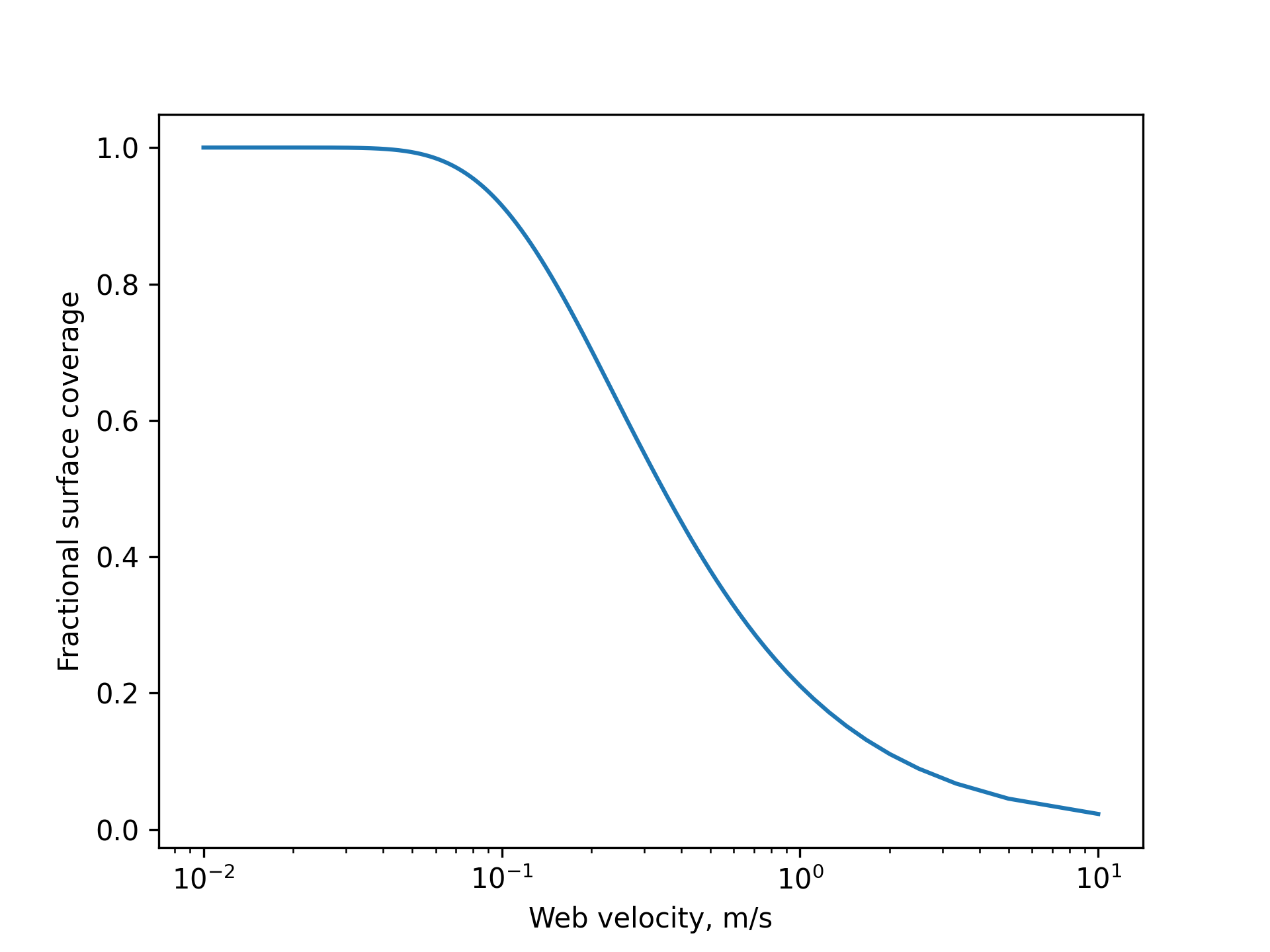
Saturation curve for the SpatialWellMixed model showing coverage vs web velocity.

ALD in high aspect ratio vias

Note

The KnudsenVia model is currently implemented for ALD surface kinetics with a single reaction pathway only. Use ALDchem for the surface chemistry definition.

Model for ALD coating inside high aspect ratio circular vias using Knudsen diffusion transport. The model solves the coupled diffusion-reaction equations to predict coverage profiles along the via depth as a function of exposure time.

from aldsim import Precursor, ALDchem
from aldsim.models import KnudsenVia
import matplotlib.pyplot as pt

# Define a precursor (TMA with molecular mass in g/mol)
tma = Precursor('TMA', mass=144.17)

# Define surface kinetics with ideal Langmuir behavior
kinetics = ALDchem(prec=tma, nsites=1e19, p_stick1=0.01)

# Create the KnudsenVia model at 200°C, 10 Pa, and aspect ratio 200
model = KnudsenVia(chem=kinetics, T=473.15, p=10, AR=200)

# Generate the saturation curve
time, z, coverage = model.saturation_curve()

# Plot coverage profiles at different times
for t, c in zip(time, coverage):
    pt.plot(z, c, label=("%4.2f s" % t))

pt.xlabel("Depth z/d")
pt.ylabel("Coverage")
pt.legend()
pt.show()

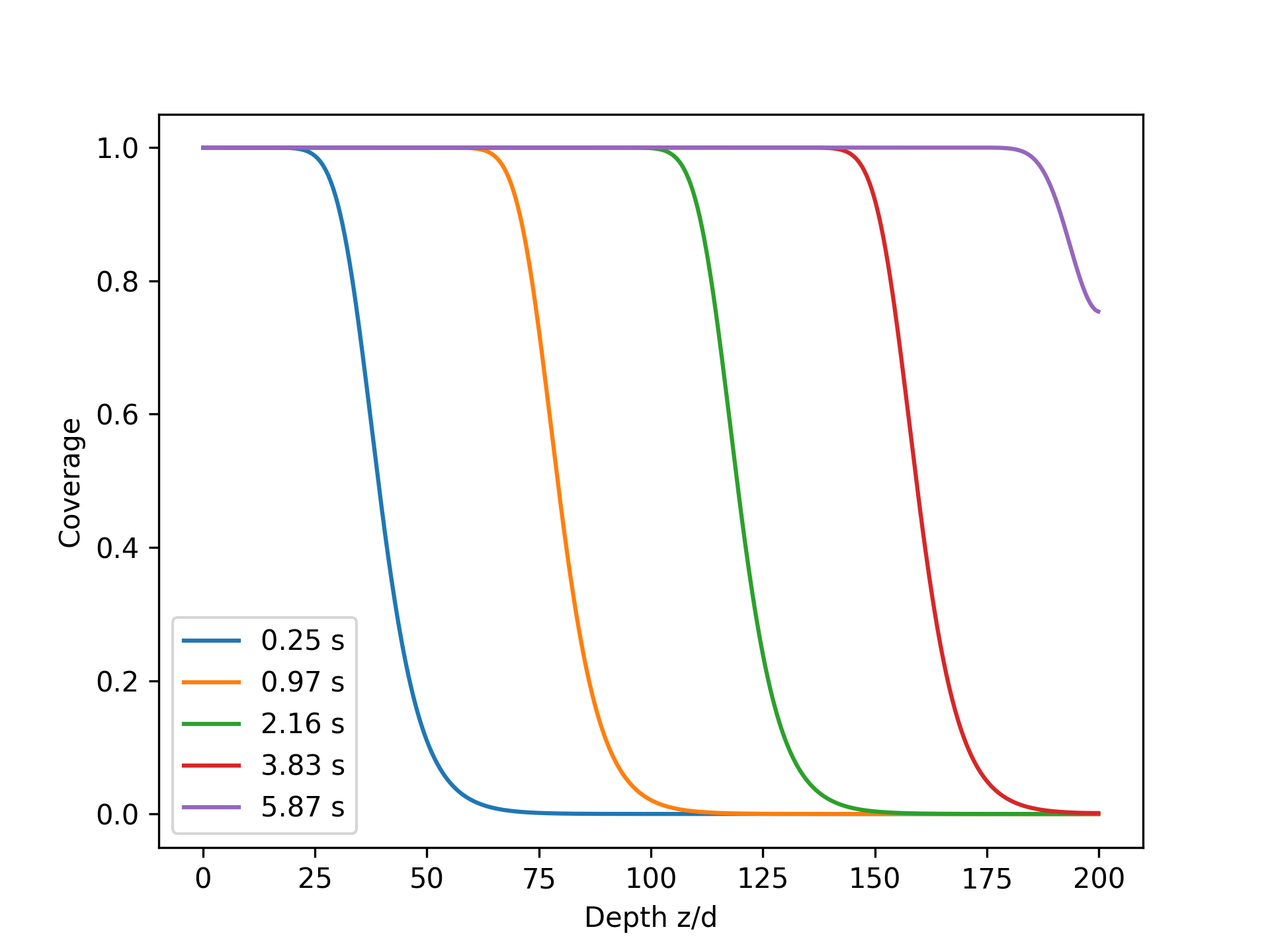
Saturation profiles as a function of normalized depth (z/diameter) for increasing dose times